Visualizing Covid-19 trends

Many websites and news outlets provide coverage and analysis of Covid-19 trends. Graphs and maps are among the best way to convey them, but I can never find the combination of data most interesting to me. Google, for example, has great tools to show changes over time at the county, state, and national levels; but the comparison of regions against each other is limited and clunky. The Johns Hopkins Covid Dashboard meanwhile has heatmaps for easily seeing how regions compare against each other, but the data are only a single and recent snapshot. One of NPR’s most interesting graphs overlays the new cases in all 50 states, but does so with logistical scales that show daily new cases as a function of total cases rather than calendar date; and only one state may be compared against just New York at a time.

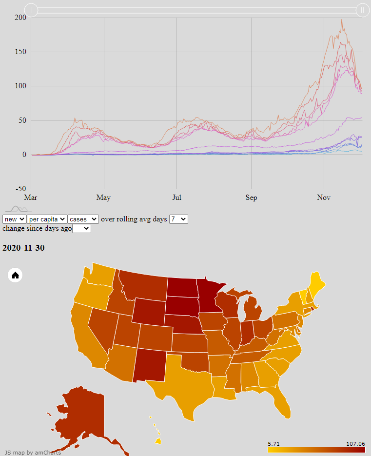
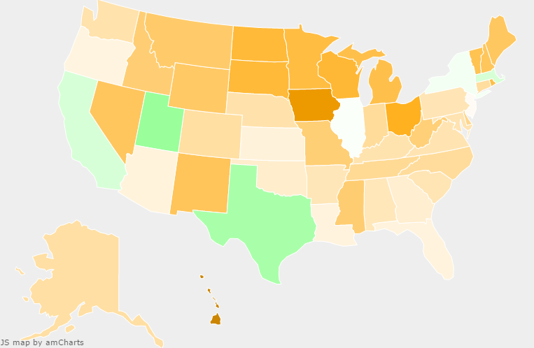
I set out to improve the situation for myself by rendering the raw CDC data, updated daily, with my own choice of axes and metrics. The publicly available result is an interactive combination of a line graph and heat map, both powered by amCharts, which mutually update each other’s state. The user may select which core data set to draw from, how to aggregate that data, and then either which date to focus on or which two states to compare. Most significantly, the line graph plots the median and the top- and bottom-five states — key percentiles — for a given data aggregation to show how outlier states change in both value and identity over time.

The default view shows the rolling 7-day average of new cases per 100,000 residents in each state. The top graph shows the daily top- and bottom-5 states as well as the median state sandwiched between them. The heat map below shows all states on a given day.

Continue reading “Visualizing Covid-19 trends”

official 2016 registration numbers corroborate Democratic disaffection

Trump’s upset victory over Clinton last year surprised just about everyone. Particularly since he lost the popular vote by nearly 3 million ballots, I wanted to see how that election compared to other recent ones to better understand how much of an outlier Trump’s victory was. To more fairly compare election results across their different electorates, I wanted to normalize the vote share won by each party, and I chose to do it by dividing votes cast into the number of registered voters for each state [1]. The Census Bureau aggregates that registration data for each federal election, but the result for a given election isn’t certified and published until well into the following year.

I experimented with several regression techniques on the historical registration figures to approximate the 2016 result and ultimately settled on a simple linear regression for the analysis. In May of this year, the Census Bureau released the official registration data and I’ve now been able to calculate the actual vote share. It appears that the regression approach was a relatively accurate predictor, which further corroborates my earlier claim that a widespread “enthusiasm gap” primarily hurt Democrats in 2016.

Continue reading “official 2016 registration numbers corroborate Democratic disaffection”

techniques for comparing relative election turnout

Earlier this month I published a deep dive into the evolution of presidential elections in the 21st elections. The primary motivation for that, aside from better understanding the shocking result of Trump’s victory over Clinton, was to analyze the widely made observation that Clinton won the popular vote by a particularly large number of votes. Around the time of that publication, updated vote tallies from a few large states (California, New York, and to a much smaller extent Pennsylvania) allowed for another shocking headline: Clinton won more votes than Obama did in 2012.

That headline (correct though it was by 90,000 votes, or 0.15% more than Obama’s 2012 haul) served to further distract from the thesis of my piece, which was that Clinton’s campaign resulted in a significant relative dip in Democratic turnout across virtually all states. But amid the drumbeat of considering absolute vote totals across elections, one criticism of my approach was to question the utility of performing a relative analysis at all. And if it was going to be made, why choose overall voter registration to  factor significantly into that analysis? This post more thoroughly considers the motivations for and alternatives to these choices to better explain why these methods probably best help us to measure differences between presidential elections.

Continue reading “techniques for comparing relative election turnout”

Clinton’s 2016 defeat explained: a statistical analysis of 21st century presidential elections

A popular indignant refrain among certain disaffected Democrats and progressives following the disastrous 2016 election is to point out that Clinton won the popular vote. It is true that at time of writing she leads Trump by more than 2.5 million votes nationally; and that’s nearly five times the margin that Gore had over Bush in 2000, the last time the popular and electoral votes disagreed. How then could Clinton have lost the Electoral College so roundly unless it were a truly undemocratic or even sinister distortion of the popular will?

Though there certainly are valid criticisms of the Electoral College which one could use to argue against its continued existence, it turns out that the raw number of the national vote in 2016, while stunning, isn’t one of them. The furore over the disconnect in 2016 made me wonder about a far more useful measure of election turnout: vote share among registered voters, especially as compared with previous elections [1]. A rigorous statistical analysis of the available data suggest that the collapse of the Democratic coalition is alone to blame for its electoral defeat in 2016.

In this image, green means good for Democrats and orange means bad. Who do you suppose won this election?

Continue reading “Clinton’s 2016 defeat explained: a statistical analysis of 21st century presidential elections”