
Many websites and news outlets provide coverage and analysis of Covid-19 trends. Graphs and maps are among the best way to convey them, but I can never find the combination of data most interesting to me. Google, for example, has great tools to show changes over time at the county, state, and national levels; but the comparison of regions against each other is limited and clunky. The Johns Hopkins Covid Dashboard meanwhile has heatmaps for easily seeing how regions compare against each other, but the data are only a single and recent snapshot. One of NPR’s most interesting graphs overlays the new cases in all 50 states, but does so with logistical scales that show daily new cases as a function of total cases rather than calendar date; and only one state may be compared against just New York at a time.
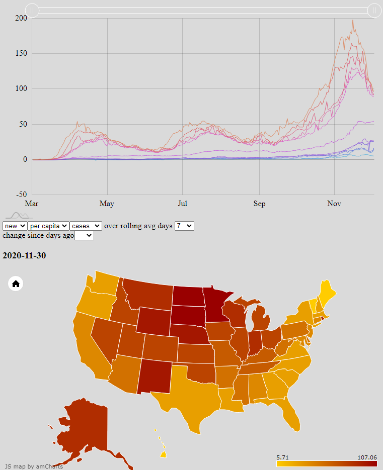
I set out to improve the situation for myself by rendering the raw CDC data, updated daily, with my own choice of axes and metrics. The publicly available result is an interactive combination of a line graph and heat map, both powered by amCharts, which mutually update each other’s state. The user may select which core data set to draw from, how to aggregate that data, and then either which date to focus on or which two states to compare. Most significantly, the line graph plots the median and the top- and bottom-five states — key percentiles — for a given data aggregation to show how outlier states change in both value and identity over time.
Analysis to date
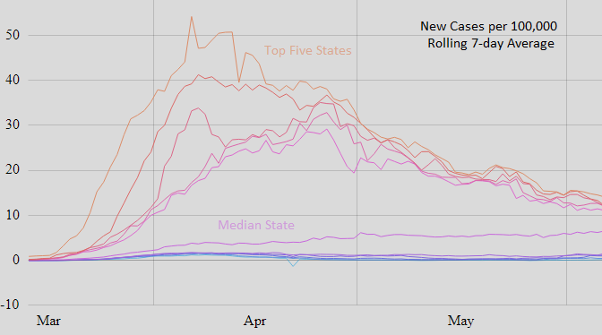
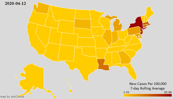
The key question in my mind is essentially the Covid “mood” of the US over time. That mood is defined by how hotspots develop and evolve. Critically, it should be normalized by regional population to enable a relative comparison. The best metric then, in my view, is the per capita new cases. As is common in many reported visualizations, the best results are usually had from rolling averages across a few days or weeks due to choppiness in recording, reporting, and aggregation from across the country.
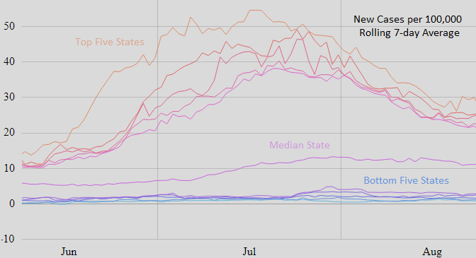
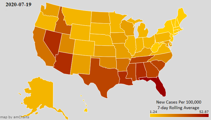
The widely-reported spikes in April and July are clearly visible from the rise and fall of new cases in the top-five states over those periods. One key finding is that the median state rose with those outbreaks but didn’t substantially fall back along with them afterward. This tells me that regional outbreaks never really recovered or subsided, but simply migrated. As Dr. Fauci said in late October, the first wave never ended.
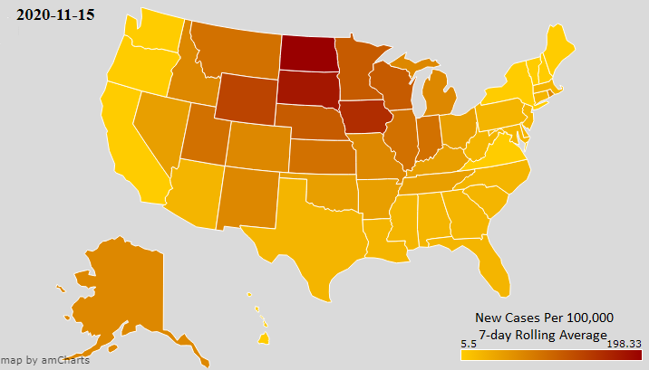
Of course the most recent spike dwarfs the first two to a shocking degree: a factor of about four times. The experts had all been predicting for months that the winter would be rough, but it was visually clear from per capita new cases by the first week in October that even the fall was headed for trouble. The dire warnings of Christmastime funerals don’t seem so hyperbolic and might have staved off disaster: those trends slack off only about a week before Thanksgiving.
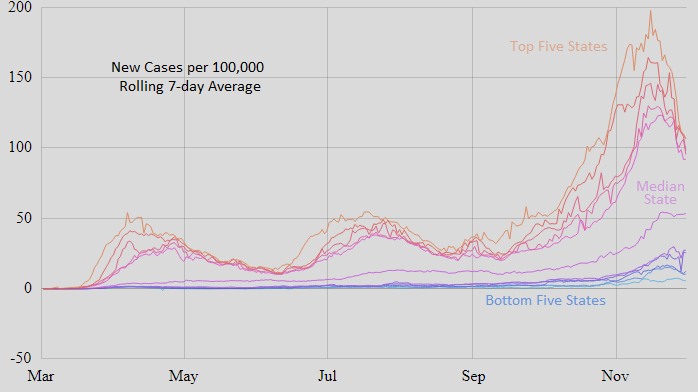
So, what will happen in the wake of Thanksgiving? Maybe we’ll be saved another huge spike after this November wakeup call: most of the country has now been through a local wringer at one point or another.
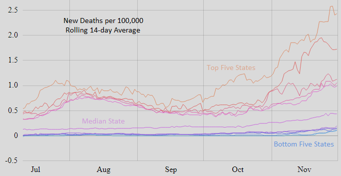
But there’s new warning sign now: per capita deaths are on the rise. Deaths were high in the spring before much was known about how the treat Covid-19 at scale, but by the summer that situation had become more manageable. Now reports are increasing of hospitals becoming overwhelmed. While that isn’t very surprising given the characteristics of the fall surge, it does make clear the stark risk of the winter ahead.
Anticipate the news
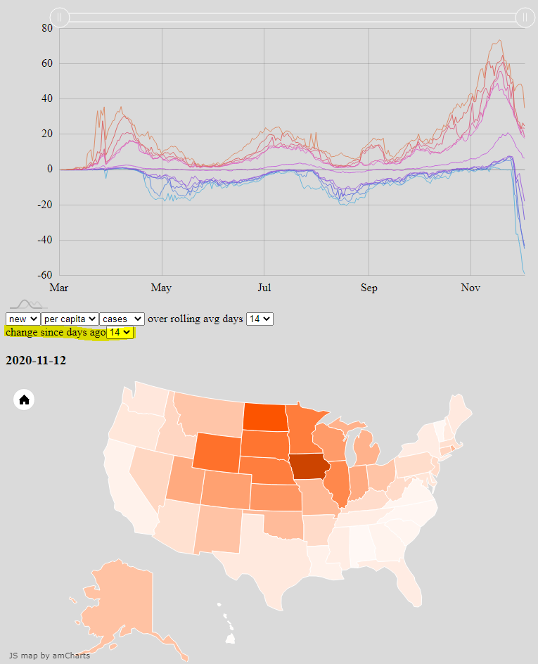
The most useful aspect of these graphs is seeing trends as they’re unfolding. Often they’ve helped me anticipate news stories by making some states’ trends visually obvious. For example, the Dakotas were clearly off the rails by September, long before this was widely reported after it got really bad in November. And it was easy to see that Iowa was skewing the same direction in the weeks before Thanksgiving, a notion the Atlantic has just covered. Rhode Island surged past the median state for per capita new cases before Halloween, so I was unsurprised to hear they were opening field hospitals after Thanksgiving.
Another good way to spot outliers is by how fast new cases are changing week over week. For this, choose to graph the change from some number of days ago: positive values indicate an increase in the value, negative ones a drop. NPR reported in mid-November that cases were “growing at record speed”, and this view makes it easy to see that we reached that condition in late October. By the first of November all states had surpassed the July surge in new cases; by the time of that reporting, no state had posted a drop in the new case rate for three weeks, a new record for the pandemic.
Play with the data yourself
Finally, some general usability notes for the visualization:
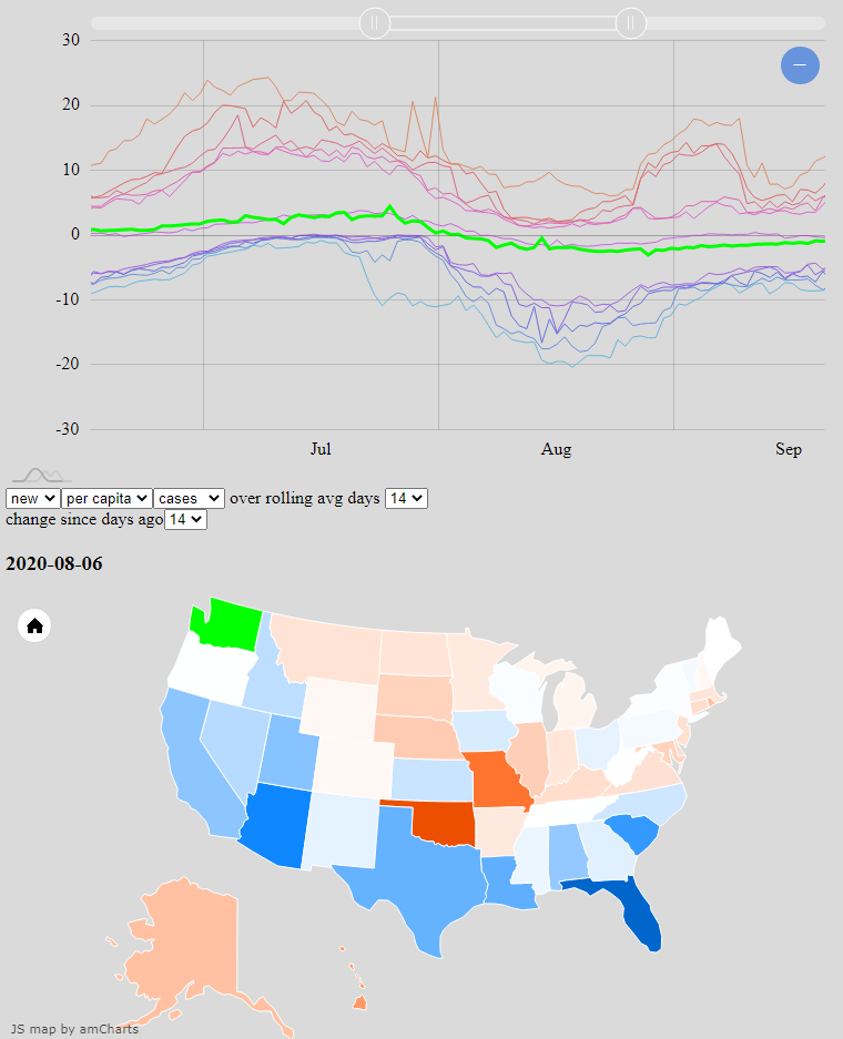
Use the slider bar at the top of the graph to zoom in on a time range. Mouse over the graph to highlight the date at your pointer, including tooltips to call out values for the top five states (A through E), the median state (M), and the bottom five states (V through Z).
Mouse over states in the heat map to plot the graph for that state against the dynamic percentiles. Click a state to pin that state’s graph to facilitate state-to-state comparisons. Click the same state again to dismiss the pin. A pinned state will also have a tooltip value when mousing over the graph.
And an overview of the available data views:
- New / Total – Switch between new data (reported daily) and total data (a cumulative total from the beginning of record keeping).
- Absolute / Per Capita – Switch between absolute numbers and state-by-state per capita normalizations. Per capita is per 100,000 residents as estimated by the Census Bureau this year. (Update: the screenshots were all based off the earlier 2019 estimates before the 2020 ones became available in late December.)
- Cases / Deaths – Switch between data about infections and deaths due to Covid-19.
- Over Rolling Average Days – Each data point is an average of this many days before and including that date. A rolling average of 1 day is just the daily raw data (no averaging).
- Change Since Days Ago – Each data point is actually the difference between that date’s value and the value from this many days ago. That includes when using a rolling average to render data. For example, the 14-day rolling average with the change since 14 days ago is actually the average of the past two weeks less the average of the two weeks before that. Dismiss this “delta” view by setting the drop down to the empty value.
Once again, the source of this data is the CDC’s daily tracker data. Other data sets exist, for example that of the Covid Tracking Project. That dataset would be particularly interesting to consume, if it were robust. It includes hospitalization and test positivity rates, for example. But the data are spotty: each day’s data come with a varying letter grade for their relative quality (e.g. C-); and entire states are consistently missing from some of the measures. At last check, there are no data for hospitalizations on any day for Alaska, California, Delaware, Iowa, Illinois, Louisiana, Michigan, Missouri, North Carolina, Nevada, Pennsylvania, Texas, Vermont, West Virginia, and the District of Columbia. That’s more than two fifths of the entire country by population.
Happy sleuthing, and may robust science and personal responsibility — both informed by clear and consistent data — save us all.